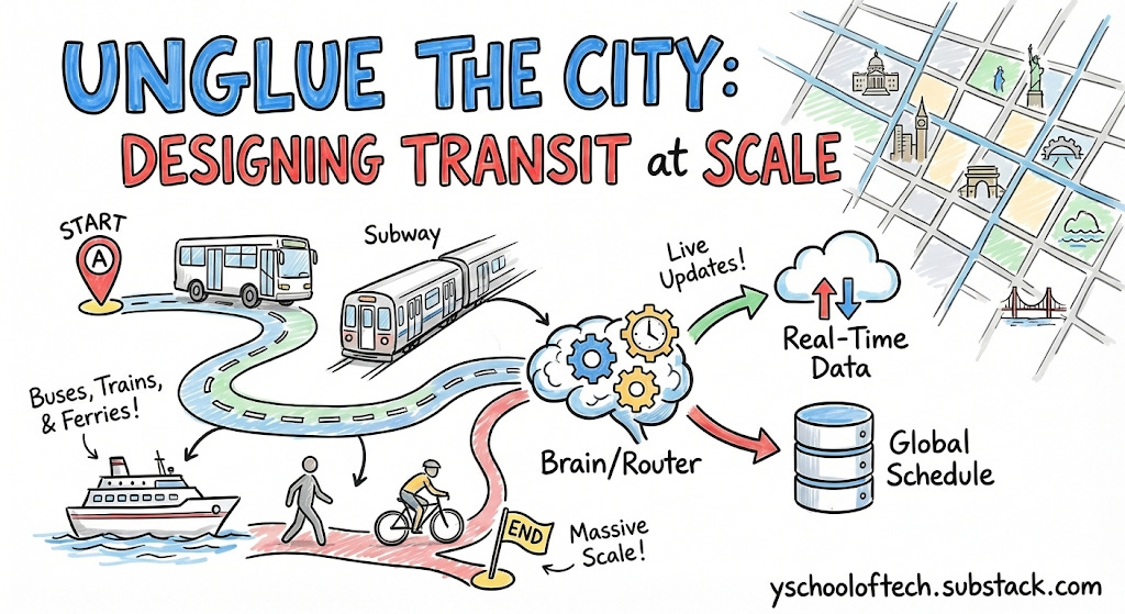
System Design Interview #4: Designing public Transit navigation (Google Maps)
How does Google Maps actually work? A deep dive into the engineering of public transit.

This is a System Design Interview question recently asked at Google
Design a system that can navigate from point A to point B using public transportation (buses, trains, ferrries tc. - anything with a time table)
1. Clarifying Questions
Ambiguity is the trap. In system design interviews, the initial prompt is deliberately vague. The interviewer isn’t just testing your technical skills; they are evaluating your ability to gather requirements and define the problem scope.
Interviewers judge you on this criteria as well. This is one competency which they evaluate too.
Scope: Is this for a single city or global?
Interviewer: Global, but assume regional sharding is acceptable.
Modality: Do we support multi-modal mixing (Walk → Bus →Train → Walk)?
Interviewer: Yes, “First Mile/Last Mile” walking is critical.
Real-Time: Do we handle live delays (GTFS {General Transit Feed Specification}-Realtime) or just static schedules?
Interviewer: Must support real-time delays. Updates must reflect within 30 seconds.
Objective Function: Are we just minimizing time?
Interviewer: Minimize arrival time AND number of transfers (Pareto-optimality). Users hate transferring 3 times to save 1 minute.
GTFS (General Transit Feed Specification) is the global, open standard format for public transit data, defining how agencies share schedules, routes, stops, and geographic info (like in agency.txt, stops.txt, routes.txt) in simple text files, allowing apps like Google Maps to provide trip planning and real-time updates (GTFS Realtime) for riders worldwide, making transit accessible and efficient.
2. Functional Requirements
Point-to-Point Routing: Get routes from Lat/Lon A to Lat/Lon B at a specific time.
Multi-Modal: Seamlessly stitch walking (street graph) with transit (schedule).
Real-Time Updates: Ingest vehicle delays (GTFS-RT) and adjust rankings immediately.
Pareto Optimization: Return multiple options (e.g., “Fastest” vs “Fewest Transfers”).
Lookahead: “Depart at 5:00 PM” vs “Arrive by 9:00 AM”.
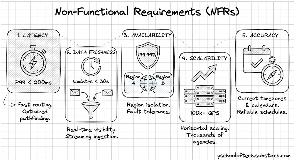
3. Non-Functional Requirements
Latency: P99 < 200ms for routing queries.
Data Freshness: Real-time updates visible to users within 30 seconds of ingestion.
Availability: 99.99% (Region-based isolation).
Scalability: Handle thousands of agencies (GTFS feeds) and 100k+ QPS.
Accuracy: Correctly handle timezones and service calendars (e.g., “Does this bus run on holidays?”).
4. Scale Estimations
Data Volume (Global):
~20,000 transit agencies globally.
~5 million stops.
~200 million scheduled stop events per day.
GTFS Static Size: 20,000 X 5MB (Avg. Data Size) ~100GB compressed.
This is small enough to fit in RAM if sharded by region (e.g., North America ~15GB).
Traffic:
User Base:
DAU (Daily Active Users): 100 Million (Approx. 10% of Google Maps users use transit).
Queries Per User: Average 2 queries/day (Morning commute, Evening commute).
Total Queries: 200 Million Queries / Day.
QPS (Queries Per Second):
Average QPS: 200M / 10^5s = 2,000 QPS.
Peak QPS (Rush Hour Multiplier): Transit is “bursty”. Everyone checks at 8:00 AM.
Assume Peak is 20 X Average.
Peak QPS: ~40,000 QPS.
Read/Write Ratio: Heavily Read-intensive (Routing). Writes (RT updates) are frequent but low volume compared to reads.
This gives you a brief idea of what is the query pattern and storage size to work on HLD.
5. Core Entities
Stop: A location where a vehicle halts (Lat/Lon).
stop_id,name,latitude,longitude,location_type,parent_stationRoute: Logical group of trips (e.g., “Line 1 Red”).
route_id,agency_id,short_name,long_name,type,colorTrip: A specific vehicle journey (e.g., “The 8:00 AM departure of Line 1”).
trip_id,route_id,service_id,trip_headsign,direction_id,realtime_delay_offsetStopTime: A specific event (Trip T arrives at Stop S at Time X).
trip_id,stop_id,arrival_time,departure_time,stop_sequenceTransfer: A foot-path between two stops (Platform A to Platform B).
from_stop_id,to_stop_id,type,min_transfer_timePattern: A sequence of stops that a trip follows. (Optimization: Group trips with the same stop sequence into a “Pattern” to scan them together).
pattern_id,route_id,stops,trips
6. API Design
GET /v1/route
Request :-
{
  "origin": "37.7749,-122.4194",
  "destination": "37.8044,-122.2711",
  "departure_time": "2024-10-05T08:00:00Z",
  "modes": ["TRANSIT", "WALK"],
  "optimization": "PARETO" // Returns fastest AND fewest transfers
}
Response: Returns a list of Itinerary objects, each containing legs (Walk Leg, Transit Leg, Walk Leg).
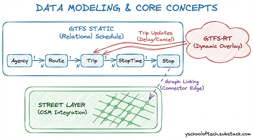
7. Data Modeling & Core Concepts
Before diving into the High-Level Design (HLD), we must understand the unique data challenges in transit. Unlike simple road networks, transit data has a temporal dimension—edges appear and disappear based on time.
We rely on two global standards: General Transit Feed Specification (GTFS) for the baseline schedule and GTFS-Realtime for live updates. However, these are interchange formats, not query formats. Our system must compile them into high-performance internal structures.
7.1 GTFS Static: The Relational Schedule
GTFS Static is a set of CSV files (tables like stops.txt, routes.txt, stop_times.txt) that define the theoretical schedule.
The Challenge: It mimics a normalized relational database.
The Solution: We cannot afford SQL joins during a pathfinding query. The ingestion pipeline must “flatten” these relations, converting ID-based references (e.g.,
stop_id) into direct memory pointers or array indices for O(1) access.
7.2 GTFS Realtime: The Dynamic Overlay
Static schedules are merely promises; the reality is often different.
The Mechanism: GTFS-Realtime uses Protocol Buffers (protobufs) to stream updates about trip delays, cancellations, and vehicle positions.
The Challenge: “Time Warping.” When a delay message arrives (e.g., “Trip A is 5 mins late”), the graph state must mutate instantly without locking the entire system for readers.
7.3 The Street Layer: Integration with OSM
Transit stops exist as isolated coordinates, but passengers start their journeys on streets.
The Source: We ingest OpenStreetMap (OSM) data to build a pedestrian routing graph.
The Engineering Challenge: Graph Linking. We must mathematically “project” every transit stop onto the nearest valid street edge. This creates a “Connector Edge” with a calculated walking cost, seamlessly stitching the street graph to the transit graph.
8. The “Aha!” Moment: Choosing the Algorithm
This section differentiates a senior engineer from a junior one. We move away from generic graph algorithms toward domain-specific optimization.
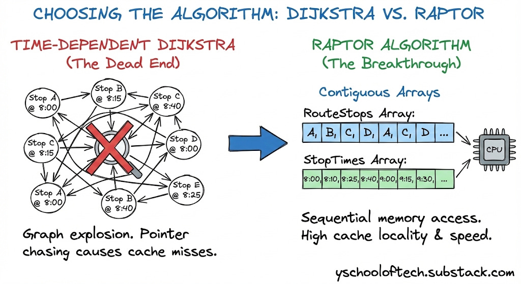
8.1 The Dead End: Time-Dependent Dijkstra
In standard road networks, Dijkstra’s algorithm is king. In transit, it fails.
The Setup: To use Dijkstra, we must build a Time-Expanded Graph. If a bus runs 50 times a day, we create 50 separate nodes for that stop (e.g.,
StopA_0800,StopA_0815).The Failure Mode:
Graph Explosion: For a major city, the node count explodes into the billions.
Memory Thrashing: The graph no longer fits in the CPU cache. Dijkstra’s algorithm randomly chases pointers (following edges), causing massive L3 cache misses. Latency spikes from milliseconds to seconds.
8.2 The Breakthrough: RAPTOR
In 2012, Microsoft Research introduced RAPTOR (Round-Based Public Transit Routing). It abandons the priority queue entirely.
The Insight: Transit optimization is not just about time; it is about the Number of Transfers. RAPTOR optimizes for transfers first.
The Algorithm Flow: RAPTOR operates in discrete “Rounds.” Round k computes the earliest arrival at every stop in the city using exactly k transfers.
Round 0: Initialize Source Stop at
t=0, all others atInfinity.Round 1: Scan all routes passing through the Source. Update arrival times at all downstream stops (0 transfers).
Round k: Identify stops that were “improved” in the previous round. Only scan routes that touch these specific marked stops.
Why it is Fast (Data-Oriented Design): RAPTOR does not use “Node” or “Edge” objects scattered in the heap. It uses flat, primitive arrays:
int[] RouteStops: A massive contiguous array of all stops.int[] StopTimes: A contiguous array of all arrival times.
Cache Locality: When the algorithm scans a route, it reads linearly through these arrays. The CPU hardware pre-fetcher anticipates this, pulling data into the L1 cache before the code even asks for it. This memory bandwidth optimization makes RAPTOR 10x-50x faster than Dijkstra for transit networks.
Interview Tip: Depth vs. Breadth
In a 1-hour system design interview, you aren’t expected to implement complex algorithms like RAPTOR from scratch. However, referencing it demonstrates strong domain knowledge.
The Key Takeaway: Simply explaining why standard Dijkstra fails (cache misses) and why RAPTOR works (array-based memory locality) is sufficient to impress the interviewer.
Deep Dive: If you want to understand the internal mechanics, you can read the full breakdown here.
9. High Level Design (HLD)
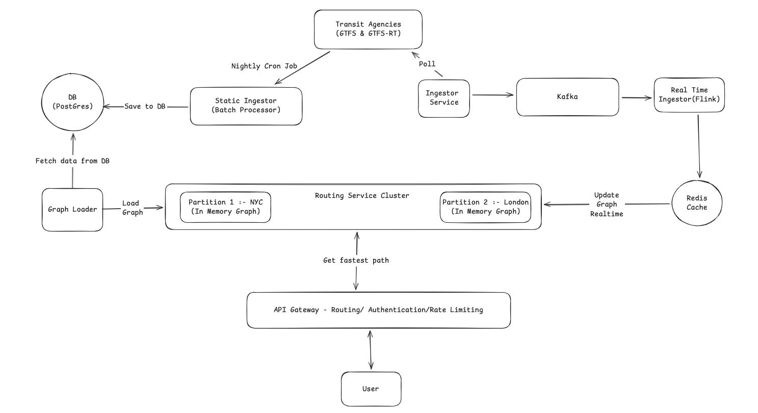
The system is designed with three clear pipelines: Static Data Processing (Offline), Real-Time Data Ingestion (Speed Layer), and the Serving Layer.
9.1 Static Data Ingestion (Offline Layer)
This process builds the foundation of our map and runs once every night.
Trigger: A Nightly Cron Job wakes up the system to start the process.
Ingest: The Static Ingestor (Batch Processor) pulls the full timetables (GTFS) from the Transit Agencies.
Store: It processes this data (cleaning and merging stops) and saves the “clean” schedule into the DB (Postgres).
Load: The Graph Loader reads the schedule from Postgres, converts it into an optimized graph format, and pushes it to the Routing Service Cluster.
9.2 Real-Time Data Ingestion
This pipeline handles live updates (like delays or cancellations) so the graph stays current.
Collect: The Ingestor Service continuously polls the Transit Agencies for live data (GTFS-RT).
Stream: It sends these raw updates to Kafka. This acts as a buffer to handle high traffic without crashing.
Process: The Real Time Ingestor (Flink) picks up the data from Kafka. It removes duplicates and formats the delay information.
Cache: Flink writes the latest status of every train/bus to the Redis Cache. This serves as the “Source of Truth” for all current delays.
9.3 The Routing Service Cluster (The Core)
This is the distributed engine that calculates the routes.
In-Memory: As shown in the diagram, the cluster keeps the entire graph in RAM for speed.
Partitions: The world is split into segments. Partition 1 handles NYC requests, while Partition 2 handles London.
Syncing: The cluster connects to the Redis Cache. When Flink updates the cache with a delay (e.g., “Subway A is late”), the graph updates its in-memory schedule in real-time.
9.4 End-to-End Flow (A User Request)
Here is what happens when a user asks: “How do I get from Times Square to the Airport?”
Find the Right Server: The system looks at the user’s location and forwards the request to the server managing that specific region.
Find Nearest Stops: The server identifies the closest transit stops to the user’s starting point and their destination.
Search: The engine scans the timetables in memory to find the best connection.
Real-Time Check: As it scans, it checks the live status. If the usual subway train is delayed, the engine sees the new, later time. It might automatically choose a different bus or train if that gets the user there faster.
Response: The best itinerary is sent back to the user’s phone.
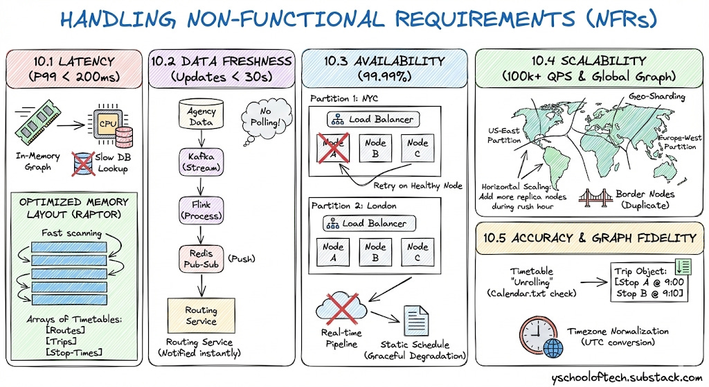
10. Handling Non-Functional Requirements (NFRs)
10.1 Latency (P99 < 200ms)
To achieve sub-200ms response times, we eliminate slow database lookups during the user request.
In-Memory Graph: The Routing Service Cluster loads the data entirely into RAM. Accessing RAM takes nanoseconds, whereas querying a database takes milliseconds.
Optimized Memory Layout (RAPTOR): We do not use a standard graph where every departure is a separate node (which would create billions of nodes). Instead, we organize the graph as arrays of Timetables (Routes, Trips, and Stop-Times). This compact structure allows the CPU to scan routes extremely fast.
10.2 Data Freshness (Updates < 30s)
We ensure users see delays almost instantly.
Streaming Pipeline: We use Kafka and Flink to process updates. This is a continuous stream, meaning data moves from the agency to the routing engine in seconds.
Push Model (Pub-Sub): The Redis Pub-Sub mechanism pushes updates directly to the Routing Service. The service is notified immediately when a change happens; it does not waste time “polling” a database.
10.3 Availability (99.99%)
We ensure the system stays online even if parts fail.
Region-Based Isolation: If the “London” partition crashes due to bad data, the “NYC” partition continues to serve users without interruption.
Replication: Each partition (e.g., Partition 1: NYC) consists of multiple identical nodes behind a load balancer. If one node fails, the API Gateway instantly retries the request on a healthy node.
Fallback Strategy: If the real-time pipeline fails, the system gracefully degrades to the static schedule, ensuring users still get a route (even if it lacks delay info) rather than an error.
10.4 Scalability (100k+ QPS & Global Graph)
We handle the massive size of the world’s transit data and high user traffic through Geo-Sharding.
Graph Sharding (Data Scale): We cannot fit the entire world’s schedule into the RAM of one machine. We split the graph geographically using S2 Geometry.
Partitioning: We create distinct graph partitions (e.g.,
US-East,Europe-West). A server only loads the partition relevant to its region.Border Nodes: To handle trips between regions (e.g., a train from Paris to London), we duplicate “Border Nodes” (major hubs) in both partitions, allowing the graph to bridge the gap seamlessly.
Horizontal Scaling (Traffic Scale): The Routing Services are stateless. To handle 100k+ queries per second, we simply add more replica nodes to the busy partitions (e.g., during rush hour in NYC).
10.5 Accuracy & Graph Fidelity
We ensure the graph mathematically represents the real world, not just a drawing of lines.
Timetable “Unrolling”: The graph creation process doesn’t just draw a line between Stop A and Stop B. It unrolls the timetable.
Service Calendars: During ingestion, we check the
calendar.txtfile. If a bus only runs on “Mondays,” we generate valid trips only for Mondays.Trip Objects: We convert raw times into Trip Objects containing sorted arrays of stop times (e.g., Stop A @ 9:00, Stop B @ 9:10). The routing algorithm reads these exact arrays, ensuring we never suggest a bus that has already left.
Timezone Normalization: The Static Ingestor converts all agency times into a consistent internal format (like UTC or normalized local time) to prevent logical errors when routes cross timezone boundaries.
11. Tradeoffs & Alternatives
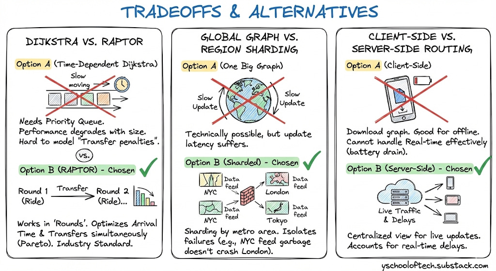
Dijkstra vs. RAPTOR
Option A (Time-Dependent Dijkstra): Needs a Priority Queue. Performance degrades as graph size grows. Hard to model “Transfer penalties”.
Option B (RAPTOR) - Chosen: Works in “Rounds” (Ride 1, Transfer, Ride 2...). It optimizes for “Arrival Time” and “Number of Transfers” simultaneously (Pareto Optimization). It is the industry standard for Transit.
Global Graph vs. Region Sharding
Option A (One Big Graph): Technically possible for just Transit (fewer nodes than road network), but update latency suffers.
Option B (Sharded) - Chosen: Sharding by metro area allows us to isolate failures. If “NYC Real-time feed” sends garbage data, it only crashes the NYC shard, not London.
Client-Side vs. Server-Side Routing
Option A (Client): Download city graph to phone. Good for offline.
Tradeoff: Cannot handle Real-time delays effectively (battery drain to sync constantly).
Choice: Server-Side. We need to account for live traffic and delays which requires a centralized view.